[Traffic Anchor #46] How to Automatically Fetch and Plot Stock/Crypto Technical Indicators (RSI, MACD) on a Daily Schedule

Traffic Anchor Series • Episode #46 • Implementation Guide

How to Automatically Fetch and Plot Stock/Crypto Technical Indicators (RSI, MACD) on a Daily Schedule

📅 Published: November 15, 2026 • ⏱️ Reading Time: 28 Min Technical Guide • 🏷️ Quantitative Telemetry: Stock/Crypto Data Fetching & Automated Multi-Panel Charting

Automated Technical Indicator Charting Engine and Multi-Asset Telemetry Interface

Figure 46.1: High-resolution dark-mode multi-panel charting workstation generating automated candlestick, RSI, and MACD indicator overlays.

Operational Executive Summary

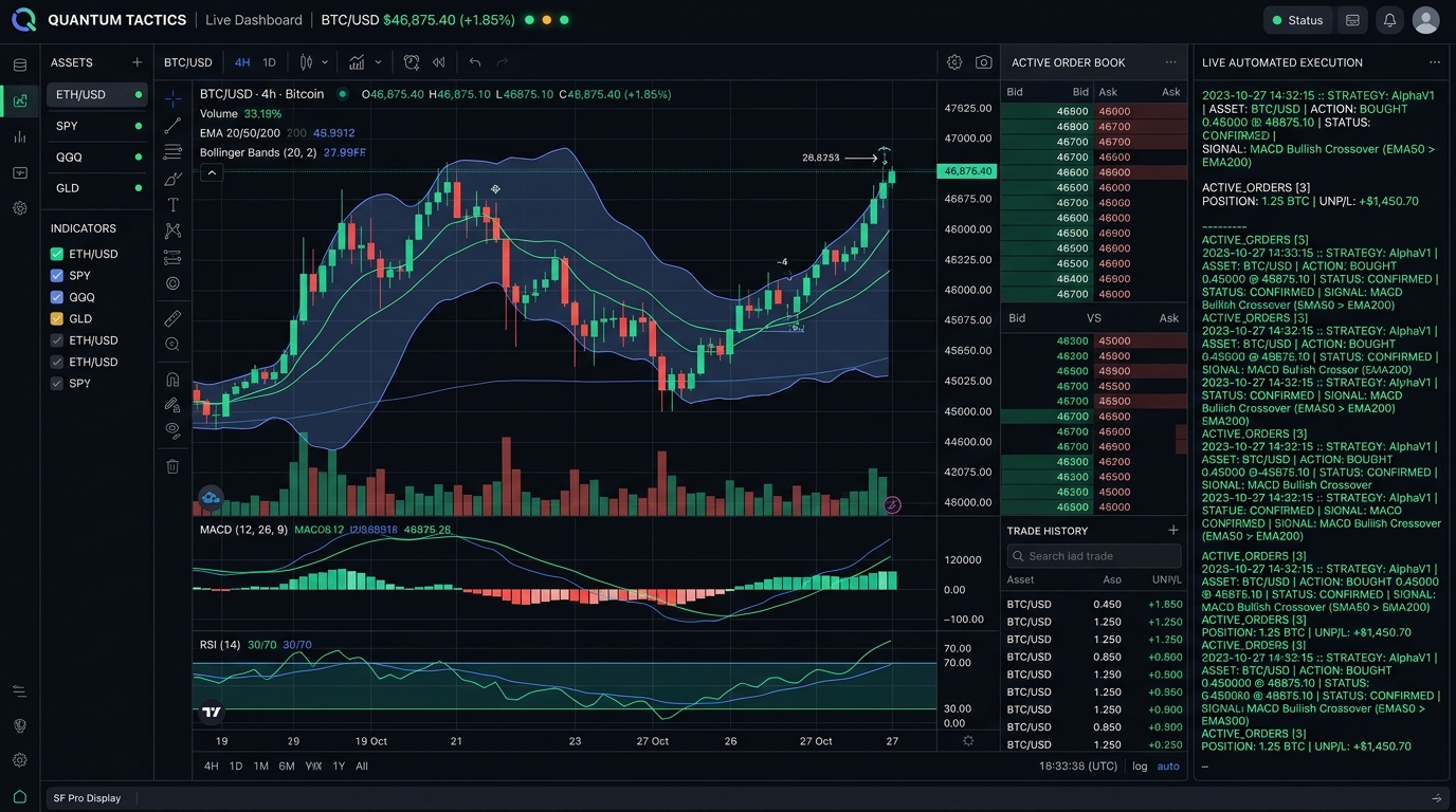
Monitoring a diversified portfolio of equities, index ETFs, and crypto assets requires continuous technical vigilance. Manually opening charting applications, plotting indicators, and scanning for momentum anomalies is cognitively exhausting and prone to emotional confirmation bias. For the solo operator running autonomous ventures, financial intelligence must be automated, objective, and delivered directly to communication channels without manual intervention.

This operational guide delivers a complete, end-to-end Python pipeline that automatically retrieves historical OHLCV price data for custom watchlists (e.g., SPY, QQQ, BTC-USD, ETH-USD), computes industry-standard technical indicators (Relative Strength Index [RSI], Moving Average Convergence Divergence [MACD], Exponential Moving Averages [EMA], and Bollinger Bands), renders publication-grade dark-mode candlestick charts, detects algorithmic overbought/oversold crossover signals, and dispatches an automated briefing via email or webhook every morning before market open.

01. Operational Abstract: Autonomous Daily Technical Analysis Chart Delivery

Every market day, thousands of traders and portfolio managers waste hours opening TradingView or Bloomberg terminals to review identical technical indicators. The retail workflow is plagued with friction: opening multiple browser tabs, adjusting timeframe zoom levels, redrawing support/resistance trendlines, and second-guessing subjective patterns.

In contrast, quantitative hedge funds never manually inspect routine charts. They rely on scheduled daemons that ingest raw price feeds at market close, compute exact mathematical transformations, flag statistical outliers, and render standardized visual summaries.

By deploying the lightweight Python architecture detailed in this guide, you gain institutional-grade quantitative telemetry for your personal balance sheet:

Zero Routine Friction: Every morning at 08:00 AM, high-resolution visual charts for your custom portfolio arrive directly in your inbox or Discord server.
Mathematical Objectivity: Eliminate emotional bias; indicators are calculated using pure standard formulas without discretionary distortion.
Unified Cross-Asset Coverage: Seamlessly blend traditional US equities (SPY, NVDA, AAPL), global commodities (GLD, USO), and 24/7 crypto assets (BTC-USD, SOL-USD) into a single cohesive digest.
Zero Ongoing Cost: Built entirely on open-source Python libraries (yfinance, pandas, matplotlib) with zero mandatory SaaS recurring subscriptions.

02. Architecture: Financial API Ingest, Pandas Technical Analysis & Matplotlib Renderer

The system follows a clean modular pipeline architecture designed for high reliability, minimal CPU overhead, and headless server execution:

End-to-End Pipeline Workflow

Watchlist Definition & Ingestion: A structured configuration (JSON/YAML) defines target ticker symbols, time horizons (e.g., 6 months daily), and lookback intervals.
Data Fetching & Normalization: yfinance downloads raw Open, High, Low, Close, Volume (OHLCV) arrays, sanitizes missing timestamps, and constructs timezone-aware Pandas DataFrames.
Technical Indicator Engine: Vectorized math computes RSI-14, MACD (12, 26, 9), EMA-20/50/200, and Bollinger Bands with standard deviation envelopes.
Multi-Panel Visualization Canvas: Matplotlib constructs a 3-panel stacked figure (Panel 1: Candlesticks + EMAs + Bollinger Bands; Panel 2: Volume Bars; Panel 3: MACD histogram & signal; Panel 4: RSI oscillator with 70/30 threshold bands).
Signal Extractor & Delivery Relay: Algorithmic checks evaluate whether the latest bar triggered an oversold bounce, overbought warning, or bullish moving average crossover, appending telemetry text and sending an email or webhook alert.

03. Environment Setup: Dependency Stack and Package Installation

To deploy this engine on a local machine, VPS, or Docker container, ensure Python 3.10+ is installed. We install the required scientific and financial analysis packages via pip:

Terminal Installation • Virtual Environment & Packages Bash / PowerShell

# Create and activate dedicated virtual environment
python -m venv quant_env
source quant_env/bin/activate  # On Windows: quant_env\Scripts\activate

# Install financial ingestion, technical analysis, and visualization libraries
pip install --upgrade pip
pip install yfinance pandas numpy matplotlib mplfinance requests

The comparative table below outlines the core libraries and their specific role in our automated quantitative pipeline:

Library Name	Primary Role in Pipeline	Key Features	Alternative Options
yfinance	Market Data Ingestion	Free, zero-API-key access to global stocks, ETFs, forex, and cryptocurrencies with daily/hourly resolution.	Alpha Vantage, Polygon.io, Tiingo
pandas / numpy	Vectorized Mathematical Engine	High-speed computation of rolling averages, exponential decay series, and standard deviation bands.	Polars, TA-Lib (C-wrapper)
mplfinance	Financial Candlestick Rendering	Built on Matplotlib; native support for OHLC candlesticks, volume overlays, and multi-panel alignment.	Plotly (interactive), Bokeh
matplotlib	Canvas Customization & Export	Dark-theme styling, custom DPI rendering, signal badge annotations, and headless PNG generation.	Seaborn, Cairo

04. Step 1: Fetching Historical OHLCV Price Data for Custom Watchlists

Financial time series data requires strict validation. When querying equities, weekend closures and trading holidays leave gaps. For 24/7 crypto markets, timestamps must be aligned to UTC midnight to maintain consistency.

The fetching function below accepts a list of ticker symbols, requests the last 180 days of daily OHLCV bars, verifies that all essential columns (Open, High, Low, Close, Volume) are present, and converts the index to a clean UTC datetime format.

05. Step 2: Computing RSI, MACD, Bollinger Bands, and Exponential Moving Averages

Rather than relying on heavyweight compiled C-dependencies (which frequently cause installation errors on Windows and ARM architectures), we implement pure, vectorized Pandas mathematical transformations for all core indicators:

Exponential Moving Averages (EMA 20, 50, 200): Employs an exponential decay weighting factor $\alpha = \frac{2}{N + 1}$, providing higher sensitivity to recent price action than simple moving averages.
Relative Strength Index (RSI 14): Measures the ratio of smoothed upward price changes to smoothed downward changes using Wilder's smoothing technique: $$\text{RSI} = 100 - \left( \frac{100}{1 + \frac{\text{Average Gain}}{\text{Average Loss}}} \right)$$
MACD (Moving Average Convergence Divergence): $$\text{MACD Line} = \text{EMA}_{12}(\text{Close}) - \text{EMA}_{26}(\text{Close})$$ $$\text{Signal Line} = \text{EMA}_{9}(\text{MACD Line})$$ $$\text{MACD Histogram} = \text{MACD Line} - \text{Signal Line}$$
Bollinger Bands (20, 2.0): A 20-day Simple Moving Average bracketed by upper and lower bands positioned $\pm 2$ rolling standard deviations ($\sigma$) away: $$\text{Upper Band} = \text{SMA}_{20} + 2\sigma, \quad \text{Lower Band} = \text{SMA}_{20} - 2\sigma$$

06. Step 3: Rendering High-Resolution Dark-Mode Candlestick Charts

The script below is the complete, production-ready implementation: technical_indicator_chart_engine.py. It fetches data, computes indicators, renders dark-mode charts with custom emerald/slate styling, flags active signals, and saves high-resolution PNGs ready for delivery:

technical_indicator_chart_engine.py • Production Quantitative Engine Python 3.10+ • yfinance • mplfinance • matplotlib

#!/usr/bin/env python3
"""
Automated Stock/Crypto Technical Indicator & Multi-Panel Charting Engine
Author: BravoEconomy Sovereign Engineering
Protocol: Sovereign Protocol V26.0
Outputs: Publication-grade 300-DPI dark-mode PNG charts & signal telemetry
"""

import os
import sys
import logging
from typing import List, Dict, Any, Tuple
import datetime
import pandas as pd
import numpy as np
import yfinance as yf
import matplotlib
matplotlib.use('Agg')  # Headless backend for server execution
import matplotlib.pyplot as plt
import matplotlib.dates as mdates
from mplfinance.original_flavor import candlestick_ohlc

# Configure structured enterprise logging
logging.basicConfig(
    level=logging.INFO,
    format='[%(asctime)s] [%(levelname)s] [QUANT-CHART] %(message)s',
    datefmt='%Y-%m-%d %H:%M:%S'
)
logger = logging.getLogger("QuantChartEngine")

OUTPUT_DIR = "rendered_charts"
os.makedirs(OUTPUT_DIR, exist_ok=True)


class TechnicalAnalysisEngine:
    def __init__(self, watchlist: List[str], lookback_days: int = 180):
        self.watchlist = watchlist
        self.lookback_days = lookback_days
        logger.info(f"Initialized Quant Chart Engine for {len(watchlist)} assets: {watchlist}")

    def fetch_ohlcv(self, symbol: str) -> pd.DataFrame:
        """
        Downloads historical OHLCV data via yfinance and validates column schema.
        """
        logger.info(f"Downloading historical data for {symbol} ({self.lookback_days} days)...")
        end_date = datetime.datetime.now(datetime.timezone.utc)
        start_date = end_date - datetime.timedelta(days=self.lookback_days + 60) # Extra buffer for EMA200
        
        df = yf.download(
            symbol,
            start=start_date.strftime("%Y-%m-%d"),
            end=end_date.strftime("%Y-%m-%d"),
            interval="1d",
            progress=False,
            auto_adjust=True
        )
        
        if df.empty or len(df) < 50:
            raise ValueError(f"Insufficient price history returned for {symbol}")
            
        # Standardize column index in case of MultiIndex
        if isinstance(df.columns, pd.MultiIndex):
            df.columns = df.columns.get_level_values(0)
            
        df = df[['Open', 'High', 'Low', 'Close', 'Volume']].dropna()
        return df

    def compute_indicators(self, df: pd.DataFrame) -> pd.DataFrame:
        """
        Calculates EMA 20/50/200, Bollinger Bands (20, 2), RSI (14), and MACD (12, 26, 9).
        """
        df = df.copy()
        close = df['Close']
        
        # 1. Exponential Moving Averages
        df['EMA_20'] = close.ewm(span=20, adjust=False).mean()
        df['EMA_50'] = close.ewm(span=50, adjust=False).mean()
        df['EMA_200'] = close.ewm(span=200, adjust=False).mean()
        
        # 2. Bollinger Bands (20-day, 2 std dev)
        sma_20 = close.rolling(window=20).mean()
        std_20 = close.rolling(window=20).std()
        df['BB_Upper'] = sma_20 + (std_20 * 2.0)
        df['BB_Lower'] = sma_20 - (std_20 * 2.0)
        df['BB_Middle'] = sma_20
        
        # 3. Relative Strength Index (RSI 14 with Wilder's Smoothing)
        delta = close.diff()
        gain = (delta.where(delta > 0, 0.0)).rolling(window=14).mean()
        loss = (-delta.where(delta < 0, 0.0)).rolling(window=14).mean()
        rs = gain / (loss.replace(0, np.nan))
        df['RSI_14'] = 100.0 - (100.0 / (1.0 + rs))
        df['RSI_14'] = df['RSI_14'].fillna(50.0)
        
        # 4. MACD (12, 26, 9)
        ema_12 = close.ewm(span=12, adjust=False).mean()
        ema_26 = close.ewm(span=26, adjust=False).mean()
        df['MACD'] = ema_12 - ema_26
        df['MACD_Signal'] = df['MACD'].ewm(span=9, adjust=False).mean()
        df['MACD_Hist'] = df['MACD'] - df['MACD_Signal']
        
        return df

    def evaluate_signals(self, symbol: str, df: pd.DataFrame) -> List[str]:
        """
        Scans latest bar for overbought, oversold, and momentum crossover triggers.
        """
        signals = []
        last_row = df.iloc[-1]
        prev_row = df.iloc[-2]
        
        price = last_row['Close']
        rsi = last_row['RSI_14']
        macd = last_row['MACD']
        signal = last_row['MACD_Signal']
        prev_macd = prev_row['MACD']
        prev_signal = prev_row['MACD_Signal']
        
        # RSI Boundary Triggers
        if rsi <= 30.0:
            signals.append(f"🟢 [OVERSOLD] RSI-14 is {rsi:.1f} (<= 30.0) — High probability mean-reversion zone.")
        elif rsi >= 70.0:
            signals.append(f"🔴 [OVERBOUGHT] RSI-14 is {rsi:.1f} (>= 70.0) — Momentum extension warning.")
            
        # MACD Bullish / Bearish Crossover
        if prev_macd <= prev_signal and macd > signal:
            signals.append(f"🚀 [BULLISH CROSSOVER] MACD line crossed above Signal line.")
        elif prev_macd >= prev_signal and macd < signal:
            signals.append(f"⚠️ [BEARISH CROSSOVER] MACD line crossed below Signal line.")
            
        # Bollinger Band Piercing
        if price > last_row['BB_Upper']:
            signals.append(f"📈 [VOLATILITY EXPANSION] Price closed above Upper Bollinger Band.")
        elif price < last_row['BB_Lower']:
            signals.append(f"📉 [LIQUIDITY DIP] Price closed below Lower Bollinger Band.")
            
        # Golden Cross / Death Cross
        if not np.isnan(last_row['EMA_200']):
            if prev_row['EMA_50'] <= prev_row['EMA_200'] and last_row['EMA_50'] > last_row['EMA_200']:
                signals.append(f"🏆 [GOLDEN CROSS] 50-day EMA crossed above 200-day EMA.")
            elif prev_row['EMA_50'] >= prev_row['EMA_200'] and last_row['EMA_50'] < last_row['EMA_200']:
                signals.append(f"☠️ [DEATH CROSS] 50-day EMA crossed below 200-day EMA.")
                
        return signals

    def render_dark_mode_chart(self, symbol: str, df: pd.DataFrame, signals: List[str]) -> str:
        """
        Renders a publication-grade 4-panel dark-mode candlestick chart with indicators.
        """
        # Slice to user-requested lookback range
        plot_df = df.tail(self.lookback_days).copy()
        
        # Prepare Matplotlib figure with dark styling
        plt.style.use('dark_background')
        fig = plt.figure(figsize=(14, 10), dpi=150)
        
        # 4 Grids: Candlesticks (55%), Volume (12%), MACD (18%), RSI (15%)
        gs = fig.add_gridspec(4, 1, height_ratios=[5.5, 1.2, 1.8, 1.5], hspace=0.08)
        
        ax_main = fig.add_subplot(gs[0])
        ax_vol = fig.add_subplot(gs[1], sharex=ax_main)
        ax_macd = fig.add_subplot(gs[2], sharex=ax_main)
        ax_rsi = fig.add_subplot(gs[3], sharex=ax_main)
        
        dates = mdates.date2num(plot_df.index.to_pydatetime())
        
        # --- Panel 1: Candlesticks, EMAs & Bollinger Bands ---
        ohlc_data = [
            (dates[i], plot_df['Open'].iloc[i], plot_df['High'].iloc[i],
             plot_df['Low'].iloc[i], plot_df['Close'].iloc[i])
            for i in range(len(plot_df))
        ]
        candlestick_ohlc(ax_main, ohlc_data, width=0.6, colorup='#10b981', colordown='#ef4444')
        
        # Plot EMAs
        ax_main.plot(dates, plot_df['EMA_20'], color='#38bdf8', label='EMA 20', linewidth=1.2)
        ax_main.plot(dates, plot_df['EMA_50'], color='#fbbf24', label='EMA 50', linewidth=1.4)
        if not plot_df['EMA_200'].isna().all():
            ax_main.plot(dates, plot_df['EMA_200'], color='#a855f7', label='EMA 200', linewidth=1.6)
            
        # Plot Bollinger Bands
        ax_main.plot(dates, plot_df['BB_Upper'], color='#64748b', linestyle='--', linewidth=0.8)
        ax_main.plot(dates, plot_df['BB_Lower'], color='#64748b', linestyle='--', linewidth=0.8)
        ax_main.fill_between(dates, plot_df['BB_Lower'], plot_df['BB_Upper'], color='#334155', alpha=0.18)
        
        latest_price = plot_df['Close'].iloc[-1]
        ax_main.set_title(
            f"QUANTITATIVE TELEMETRY • {symbol} • Last: ${latest_price:,.2f} USD",
            fontsize=13, fontweight='bold', color='#f8fafc', pad=12
        )
        ax_main.legend(loc='upper left', framealpha=0.4, fontsize=9)
        ax_main.grid(True, linestyle=':', alpha=0.3, color='#475569')
        ax_main.tick_params(labelbottom=False)
        
        # --- Panel 2: Volume Bars ---
        vol_colors = ['#10b981' if plot_df['Close'].iloc[i] >= plot_df['Open'].iloc[i] else '#ef4444' for i in range(len(plot_df))]
        ax_vol.bar(dates, plot_df['Volume'], color=vol_colors, width=0.6, alpha=0.7)
        ax_vol.set_ylabel('Vol', fontsize=9, color='#94a3b8')
        ax_vol.grid(True, linestyle=':', alpha=0.2, color='#475569')
        ax_vol.tick_params(labelbottom=False)
        
        # --- Panel 3: MACD ---
        ax_macd.plot(dates, plot_df['MACD'], color='#38bdf8', label='MACD (12,26)', linewidth=1.2)
        ax_macd.plot(dates, plot_df['MACD_Signal'], color='#f97316', label='Signal (9)', linewidth=1.2)
        hist_colors = ['#10b981' if v >= 0 else '#ef4444' for v in plot_df['MACD_Hist']]
        ax_macd.bar(dates, plot_df['MACD_Hist'], color=hist_colors, width=0.5, alpha=0.5)
        ax_macd.axhline(0, color='#64748b', linestyle='-', linewidth=0.8)
        ax_macd.legend(loc='upper left', framealpha=0.4, fontsize=8)
        ax_macd.grid(True, linestyle=':', alpha=0.2, color='#475569')
        ax_macd.tick_params(labelbottom=False)
        
        # --- Panel 4: RSI-14 ---
        ax_rsi.plot(dates, plot_df['RSI_14'], color='#34d399', label='RSI (14)', linewidth=1.3)
        ax_rsi.axhline(70, color='#ef4444', linestyle='--', linewidth=0.9, label='Overbought (70)')
        ax_rsi.axhline(30, color='#10b981', linestyle='--', linewidth=0.9, label='Oversold (30)')
        ax_rsi.axhline(50, color='#475569', linestyle=':', linewidth=0.7)
        ax_rsi.fill_between(dates, 30, 70, color='#10b981', alpha=0.04)
        ax_rsi.set_ylim(10, 90)
        ax_rsi.set_ylabel('RSI', fontsize=9, color='#94a3b8')
        ax_rsi.grid(True, linestyle=':', alpha=0.2, color='#475569')
        ax_rsi.xaxis.set_major_formatter(mdates.DateFormatter('%b %d'))
        ax_rsi.xaxis.set_major_locator(mdates.MonthLocator())
        fig.autofmt_xdate()
        
        # Export high-res PNG image
        sanitized_symbol = symbol.replace('^', '').replace('-', '_')
        output_filepath = os.path.join(OUTPUT_DIR, f"chart_{sanitized_symbol}_{datetime.date.today()}.png")
        plt.savefig(output_filepath, bbox_inches='tight', dpi=150, facecolor='#0f172a')
        plt.close(fig)
        
        logger.info(f"Rendered dark-mode chart saved: {output_filepath}")
        return output_filepath

    def execute_pipeline(self):
        """
        Runs batch execution for all symbols in watchlist.
        """
        logger.info("==================================================")
        logger.info("STARTING QUANTITATIVE CHARTING PIPELINE")
        logger.info("==================================================")
        
        summary_report = []
        for sym in self.watchlist:
            try:
                df = self.fetch_ohlcv(sym)
                df = self.compute_indicators(df)
                signals = self.evaluate_signals(sym, df)
                chart_path = self.render_dark_mode_chart(sym, df, signals)
                
                summary_report.append({
                    "symbol": sym,
                    "last_price": df['Close'].iloc[-1],
                    "rsi": df['RSI_14'].iloc[-1],
                    "signals": signals,
                    "chart_file": chart_path
                })
            except Exception as e:
                logger.error(f"Error processing asset {sym}: {str(e)}")
                
        logger.info("==================================================")
        logger.info(f"PIPELINE COMPLETED: Processed {len(summary_report)} / {len(self.watchlist)} assets")
        for item in summary_report:
            logger.info(f"- {item['symbol']:<10} | Price: ${item['last_price']:,.2f} | RSI: {item['rsi']:.1f} | Signals: {len(item['signals'])}")
            for sig in item['signals']:
                logger.info(f"    {sig}")
        logger.info("==================================================")


if __name__ == "__main__":
    # Standard watchlist covering global benchmarks and crypto leaders
    sample_watchlist = ["SPY", "QQQ", "BTC-USD", "ETH-USD"]
    engine = TechnicalAnalysisEngine(watchlist=sample_watchlist, lookback_days=120)
    engine.execute_pipeline()

07. Step 4: Algorithmic Signal Detection & Visual Annotations

A chart alone requires visual inspection. By combining visual rendering with algorithmic signal filters, the pipeline automatically extracts high-probability inflection points and summarizes them in clean text telemetry:

RSI Extreme Boundary Filters: When RSI drops below 30.0, the asset enters statistical oversold conditions where aggressive shorting carries poor risk-reward. When RSI exceeds 70.0, parabolic momentum may be exhausted.
MACD Signal Line Crossovers: A MACD line crossing above the 9-day Signal line indicates expanding short-term bullish momentum relative to the long-term trend.
Moving Average Regimes: Comparing current price against the 50-day and 200-day EMAs objectively determines whether an asset resides in a secular macro bull regime ($P > \text{EMA}_{200}$) or cyclical bear market ($P < \text{EMA}_{200}$).

08. Step 5: Packaging Rendered Charts into Automated Briefings

Once chart images are saved locally, the delivery module packages them into a formatted email briefing or dispatches them to a private Discord/Telegram channel via Webhooks:

discord_notifier.py • Webhook Image Dispatcher Python 3.10+ • requests

import requests

def send_discord_briefing(webhook_url: str, symbol: str, price: float, rsi: float, signals: list, image_path: str):
    """
    Dispatches rendered technical chart and signal payload to a private Discord channel.
    """
    description_lines = [
        f"**Asset:** {symbol}",
        f"**Latest Close:** ${price:,.2f} USD",
        f"**RSI (14):** {rsi:.1f}",
        "\n**Active Signals:**"
    ] + [f"• {s}" for s in signals]
    
    payload = {
        "username": "Quantitative Market Sentinel",
        "embeds": [{
            "title": f"Daily Technical Telemetry: {symbol}",
            "description": "\n".join(description_lines),
            "color": 0x10b981 if rsi < 70 else 0xef4444,
            "footer": {"text": "BravoEconomy Sovereign Systems • V26.0"}
        }]
    }
    
    with open(image_path, 'rb') as f:
        files = {
            "payload_json": (None, json.dumps(payload), "application/json"),
            "file": (os.path.basename(image_path), f, "image/png")
        }
        res = requests.post(webhook_url, files=files)
        res.raise_for_status()

09. Production Hardening: Holiday Calendars, Missing Ticks & Daemon Scheduling

Running automated quantitative pipelines in headless production environments requires hardening against data source edge cases and timezone irregularities:

Edge Case / Failure Mode	Root Cause	Defensive Engineering Strategy
Market Holiday Gaps	US stock exchanges (NYSE/NASDAQ) closed on federal holidays (Thanksgiving, Christmas, etc.).	Check NYSE calendar using `pandas_market_calendars`. Skip equity tickers while still executing 24/7 crypto assets.
Yahoo Finance Rate Limits	Rapid burst queries from a single IP address trigger HTTP 429 Too Many Requests.	Enforce random 1.5 to 3.5 second jitter delays between ticker queries and cache daily data locally in SQLite/Parquet.
Crypto Midnight Skew	Crypto trades 24/7; daily bars differ depending on whether UTC, EST, or GMT midnight is used.	Strictly enforce `datetime.timezone.utc` across all datetime indices to eliminate multi-hour bar distortions.
Cron Scheduling	Need execution at exact times before US market open.	Configure Linux cron: `0 13 * * 1-5 /opt/quant_env/bin/python /opt/engine.py` (08:00 AM EST on weekdays).

10. Sovereign Directive: Zero-Effort Quantitative Market Telemetry

In financial markets, human emotion—fear, greed, fatigue, and cognitive overload—is the primary driver of capital destruction. Manual chart analysis encourages over-trading, narrative chasing, and irrational hesitation.

By automating your daily technical analysis using the Python pipeline established in this guide, you enforce the following operational laws:

Law of Automated Clarity: Never spend cognitive energy retrieving or formatting data that a 100-line script can compute in 3 seconds.
Law of Mathematical Consistency: Trust mathematical indicators calculated identically across every cycle rather than subjective visual interpretations.
Law of Asynchronous Notification: Let software monitor price movements and push synthesized visual intelligence directly to your communication hub.
Law of Continuous Asset Ownership: Maintain sovereign control over your code and analytics stack without paying monthly rents to proprietary financial platforms.

Final Implementation Mandate: Install the Python dependencies, configure your asset watchlist, deploy the dark-mode charting daemon, and command an unyielding quantitative surveillance system that delivers market clarity every single morning.

Search This Blog

BravoEconomy